Applications in high voltage transmission require the analysis of electric fields that cause corona discharge, dielectric breakdown in insulators, and electromagnetic interference. The insulators that support the power lines are associated with complicated conducting structures. The simulation of a complete transmitting tower along with the power lines is fundamental for the estimation of the electric field levels at an arbitrary point on the insulators, corona rings, and in their surroundings. In this article, we will model a 3-phase, 115 kV transmission tower using a 3D electrostatic field solver.
Geometry
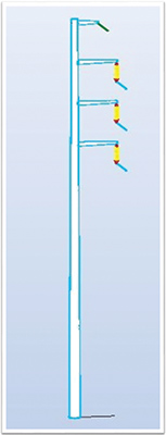
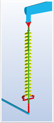
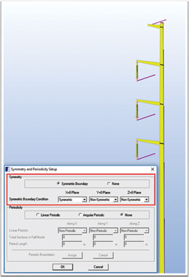
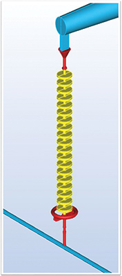
Figure 1a shows the transmission tower. This particular model was imported from a STEP file. The height of the tower is about 30 meters and there are four lines in total, phase a, phase b, phase c, and the ground wire. The power transmission lines are about one inch in diameter. The ground wire is about half an inch in diameter. All the power lines are modeled to a length of about five meters. Figure 1b shows a conductor attached to its corona ring and suspension insulator. The whole model is symmetric about the X = 0 plane. Figure 2a shows the symmetry setup and figure 2b shows the non-symmetric model. For a faster solution, we use the symmetric model.
|
|
|
|
|
|
Materials and Boundary Conditions
The tower and the conductors are made of aluminum. Since the ground wire does not carry any current, it is made of steel (linear).The insulator consists of silicone rubber sheds with a glass fiber filled nylon 6 (40%) rod in the center. The dielectric constant for these materials is calculated at the power frequency (60 Hz). The corona ring and its fixture are made of copper. The ground wire and the tower are at 0 V. The conductors along with their corona ring structures are assigned 115 kV at phase angles 0º, 120º and -120º from the top.
Meshing
This model clearly involves a wide-open space around the device, and problems involving such open regions are best handled by the Boundary Element Method (BEM). Using BEM, only the “active” regions require discretization. Fields can be calculated anywhere in 3D space. It allows for the modeling of the true geometric curvature rather than straight-line approximations. Models with thin layers and extreme aspect ratios are handled more easily. In BEM formulation, the equivalent charges that support the specified boundary conditions are found out.
From these equivalent charges, the electric potential and electric field are calculated by appropriate integration, effectively smoothing out the discretization error. BEM is more accurate and faster than a FEM-based formulation. Figures 3a and 3b show a global and local view of the 2D triangular mesh.
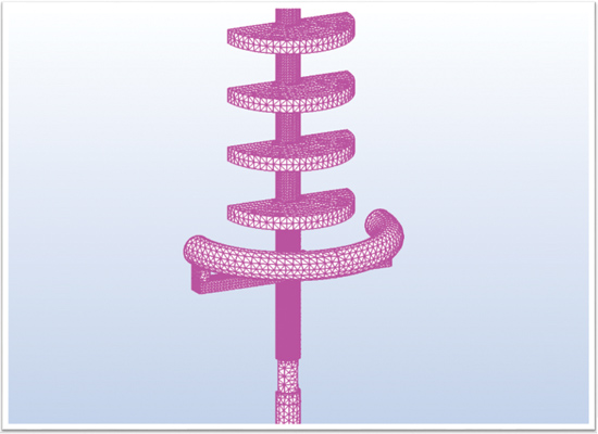
Fig. 3b. Local view of the 2D triangular mesh
Since all the materials are linear, the BEM solver needs to solve for unknowns only at the boundaries. It just requires a 2D triangular mesh on all the surfaces. You can assign the elements automatically throughout the model and refine the local mesh density manually where you need accurate results. This model contains about 101,000 2D triangular elements and requires an optimal RAM of about 14 GB. Without the symmetric conditions, this model would require about 183,000 2D elements and a RAM of about 48 GB. This is a four-fold increase in the memory requirement. It also increases the computational time significantly. Therefore, symmetry about any principal plane should be made use for a faster simulation.
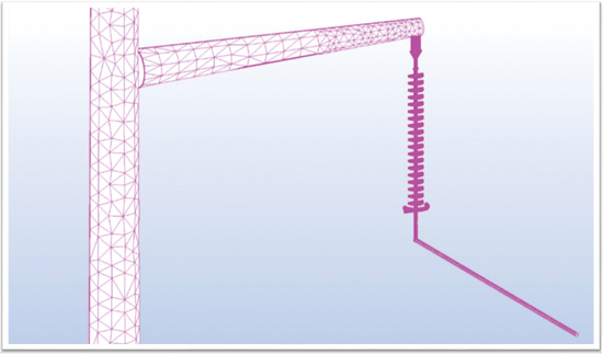
Fig. 3b. Local view of the 2D triangular mesh
Physics and Solver Settings
|
|
|
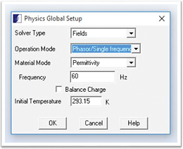
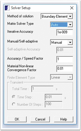
Figure 4a shows the physics settings. The solver type is set to ‘Fields’. The operation is at a single frequency of 60 Hz. Charge balance is turned off. In balanced mode, the solver will force the total charge in the model to add up to zero. In this mode, there is need for a reference potential to be set somewhere. In unbalanced mode, the surroundings around the model will hold whatever excess charge is required and the potential at infinity will be zero requiring no potential reference. Only ungrounded sources such as a battery require the charge to be balanced in the model.
Figure 4b gives the solver settings. In the solver setup, BEM is the method of solution. The matrix solver type can be set to ‘Direct’, ‘Iterative’ or ‘Auto’. In auto mode, a 3D electrostatic field solver will automatically determine the best solver without requiring any user interaction. The direct solver is robust but requires more time than the iterative solver. The meshing can be manual or self-adaptive. However, this model was meshed manually for some good local results.
Post-Processing and Results
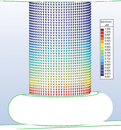
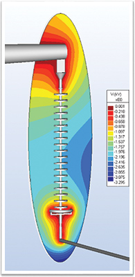
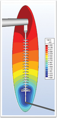
Fig. 5a. E-field without corona ring
The corona ring reduces the electric potential gradient and lowers the maximum electric field value below the corona threshold. Figures 5a and 5b show a comparison of the electric field near the bottom of an insulator with and without the corona ring. This total field at time angle 0º is directed downwards. You can observe that the maximum field reduced from about 1.05 kV/mm to 0.41 kV/mm with the corona ring.
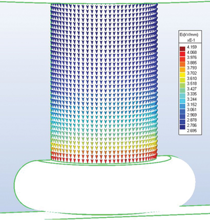
Fig. 5b. E-field with corona ring
Figure 6 shows an arrow plot of the electric field on a corona ring.
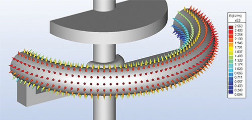
Fig. 6. Electric field on a corona ring
|
|
|
|
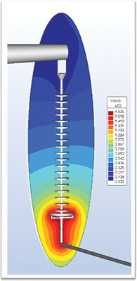
Figures 7a, 7b, and 7c show a plot of the potential contours on a plane through the mid-section of the top insulator at time angles 0º, 90º and 180º. Initially, the maximum potential near the conductor equals the peak value of line voltage as a cosine function which is square root of 2 times 115 kV i.e. 162.6 kV. At 90º, the maximum potential is 0 kV and at 180º, it is -162.6 kV. Figure 8 shows the potential contours of all three lines on the X = 0 plane.
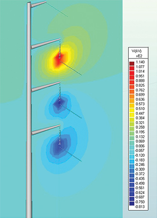
Fig. 8. Potential contours of all three lines on the X = 0 plane
To verify the simulation, we can plot the tangential electric field between two points, a, and b and calculate its line integral, which must be equal to the potential difference between the two points.
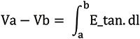
Figure 9a shows an arc is drawn from a point on the top conductor to a point on the tower. In Figure 9b, a graph of the tangential electric field is plotted and integrated along this segment. This integral equals 162 kV, which is the potential difference between the two points at time angle 0º.
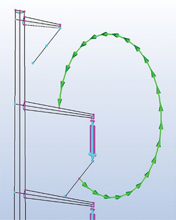
Fig. 9a. Line integral segment
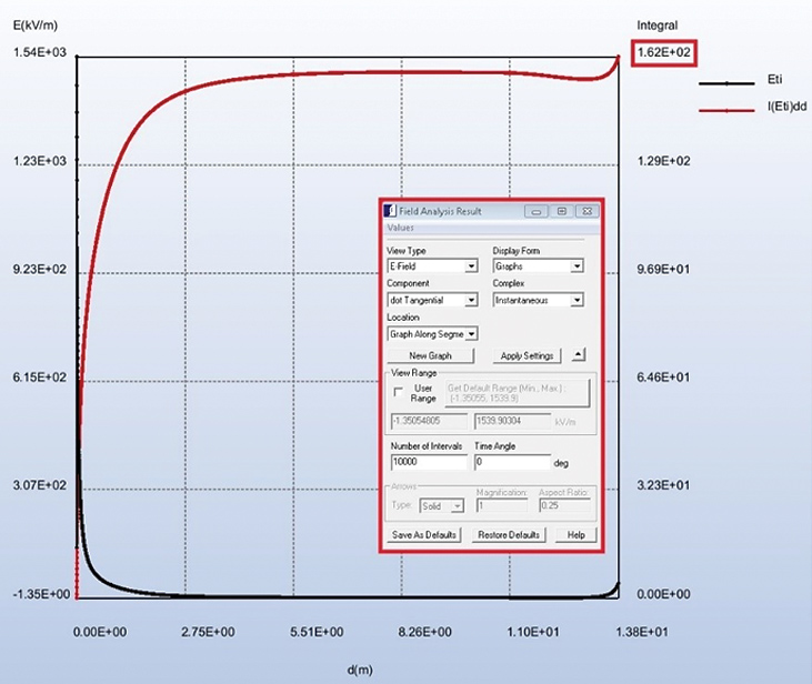
Fig. 9b. Graph of the integral
(click to enlarge)
The value of the electric field surrounding the power line must be lower than a maximum allowable limit for the safety of personnel and people on ground. A 3D electrostatic field solver can efficiently simulate these requirements. For magnetic fields, we can simulate the same model using a 3D magnetostatic field solver. The excitation here has to be the RMS value of the current flowing through these lines.
About the Author
 Dr. K.M. Prasad has been involved in developing INTEGRATED engineering software programs for the last 30 years. He obtained his Ph.D. in 1983 and is currently a member of INTEGRATED’S Technical Support Team. The focus of his work has been the simulation of real world electromagnetic field models. Dr. Prasad has considerable expertise in the minimization of the complexity of real world models without losing electromagnetic functionality. With almost three decades of experience in the simulation of electric, magnetic, thermal, and high frequency electromagnetic problems, Dr. Prasad is truly a quick trouble shooter.